Control Charts in Statistical Process Control
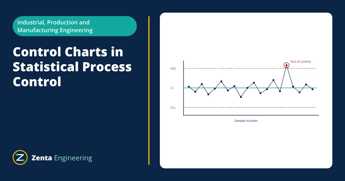
Control charts are the main tool of statistical process control (SPC). They plot a process measurement over time with a centre line and upper and lower control limits, usually at ±3 standard deviations of the plotted statistic. Points within the limits with no unusual patterns indicate common cause variation: the process is in control. Points outside the limits or non-random patterns signal special causes that should be investigated. Variables charts (X-bar and R, X-bar and S, individuals and moving range) track measurements; attributes charts (p, np, c, u) track defectives or defects.
Every process varies: no two parts are exactly the same. The question is whether the variation is the normal, predictable noise of a stable process, or a sign that something has changed: a worn tool, a new batch of material, a different operator or a drifting sensor. Control charts, developed by Walter Shewhart at Bell Laboratories in the 1920s, answer that question in real time, so problems are caught before many bad parts are made.
Common causes and special causes
- Common cause variation is inherent in the process: many small, random influences such as minor temperature fluctuations, material variation and machine vibration. Reducing it requires changing the process itself, usually a management or engineering decision.
- Special (assignable) cause variation comes from specific events: a broken tool, a wrong setting, a contaminated batch. It should be found and removed by the people running the process.
Reacting to common cause noise as if it were a special cause (tampering) actually increases variation, while ignoring special causes lets defects pile up. Control charts help tell the two apart.
Anatomy of a control chart
Types of control charts
Variables charts (measurements)
- X-bar and R chart: small subgroups (typically n = 2 to 10, often 5) are taken at regular intervals. The X-bar chart tracks subgroup means (process centring); the R chart tracks subgroup ranges (process spread).
- X-bar and S chart: uses standard deviation instead of range, better for larger subgroups (n above about 10).
- Individuals and moving range (I-MR): for one measurement at a time, such as batch processes or slow production.
- CUSUM and EWMA charts: sensitive to small, gradual shifts.
Attributes charts (counts)
- p chart: proportion defective in samples of varying size.
- np chart: number defective in samples of constant size.
- c chart: number of defects per unit of constant size, for example scratches per panel.
- u chart: defects per unit when the inspection area varies.
Control limit formulas for X-bar and R charts
With k subgroups of size n, the grand mean X̿ and average range R̄:
For n = 5, the constants are A₂ = 0.577, D₃ = 0 and D₄ = 2.114 (from standard SPC tables).
- Given
- A shaft diameter is checked in 25 subgroups of 5 parts. The grand mean is 25.012 mm and the average range is 0.020 mm. Specification is 25.00 ± 0.05 mm.
- Find
- Control limits for the X-bar and R charts, and estimate process capability Cpk.
- Assumptions
- Process stable during data collection; normal distribution; d₂ = 2.326 for n = 5 so σ = R̄ ÷ d₂.
- Solution
- X-bar UCL = 25.012 + 0.577 × 0.020 = 25.0235 mm; LCL = 25.012 − 0.0115 = 25.0005 mm
R chart UCL = 2.114 × 0.020 = 0.0423 mm; LCL = 0
σ = 0.020 ÷ 2.326 = 0.0086 mm
Cpk = min[(25.05 − 25.012), (25.012 − 24.95)] ÷ (3 × 0.0086) = 0.038 ÷ 0.0258 = 1.47 - Answer
- X-bar limits 25.0005 to 25.0235 mm, R chart UCL 0.042 mm; Cpk about 1.47, capable though slightly off centre
- Limitations
- Capability is only meaningful when the process is in statistical control; recentring to 25.000 mm would raise Cpk further.
Rules for detecting out of control signals
Besides points outside the limits, the Western Electric and Nelson rules look for non-random patterns, for example:
- One point beyond 3σ.
- Two of three consecutive points beyond 2σ on the same side.
- Four of five consecutive points beyond 1σ on the same side.
- Eight consecutive points on one side of the centre line (a shift).
- Six points in a row steadily increasing or decreasing (a trend), such as tool wear.
More rules catch smaller shifts sooner but also raise false alarms, so organisations choose a sensible set.
Implementing control charts
- Choose critical characteristics linked to customer requirements.
- Make sure the measurement system is capable (gauge R&R), since measurement error appears as process variation.
- Decide subgroup size and frequency to capture variation between, not within, subgroups.
- Collect initial data, calculate trial limits, investigate and remove special causes, and recalculate.
- Train operators to plot points and follow a reaction plan when a signal appears.
- Review charts regularly and recalculate limits after deliberate process changes.
Choosing the right chart
The choice depends on the data type and how samples are taken. If the characteristic is measured on a continuous scale, such as length, weight or temperature, and parts can be grouped into rational subgroups, use X-bar and R or X-bar and S charts. If only one measurement is available at a time, use an individuals and moving range chart. If parts are simply judged good or bad, use p or np charts, and if defects are counted on each unit, use c or u charts. When small, slow drifts matter, such as tool wear or catalyst ageing, consider EWMA or CUSUM charts.
Control charts in modern manufacturing
The value of a chart lies in the reaction to it, so every chart needs a named owner and a clear response when a signal appears.
Today, SPC software collects data directly from gauges, CMMs and machine sensors, plots charts in real time on shop floor screens and alerts engineers automatically. Control charts are also the core tool of the Control phase of Six Sigma DMAIC, and they help eliminate defects, one of the seven wastes of lean manufacturing. The same ideas apply to process plants, where variables such as temperature, pressure and flow from process instruments are monitored with control charts for consistent quality.
Frequently asked questions
What is the difference between control limits and specification limits?
Control limits are calculated from process data and show the natural variation of a stable process, typically ±3 standard deviations of the plotted statistic. Specification limits come from the customer or design and say what is acceptable. A process can be in control but still produce out of specification parts if its variation is too wide or poorly centred.
Why are control limits set at 3 sigma?
Walter Shewhart chose ±3 sigma as an economic balance. For a normally distributed statistic, only about 0.27% of points fall outside by chance, so false alarms are rare, while real shifts of meaningful size are still detected reasonably quickly.
How many samples are needed to set up a control chart?
A common guideline is at least 20 to 25 subgroups, for example 25 samples of 5 parts each, collected while the process is believed to be stable. Limits are then calculated, points outside are investigated and removed if a cause is found, and limits recalculated.
References
- W. A. Shewhart, Economic Control of Quality of Manufactured Product, Van Nostrand, 1931
- D. C. Montgomery, Introduction to Statistical Quality Control, 8th ed., Wiley
- ISO 7870-2:2023, Control charts, Part 2: Shewhart control charts
- AIAG, Statistical Process Control (SPC) Reference Manual, 2nd ed.
- Western Electric Company, Statistical Quality Control Handbook, 1956
Get one engineering email a week
New articles, worked examples and study notes every week. Free, no spam, unsubscribe any time.