Inventory Control: EOQ Model with Worked Example
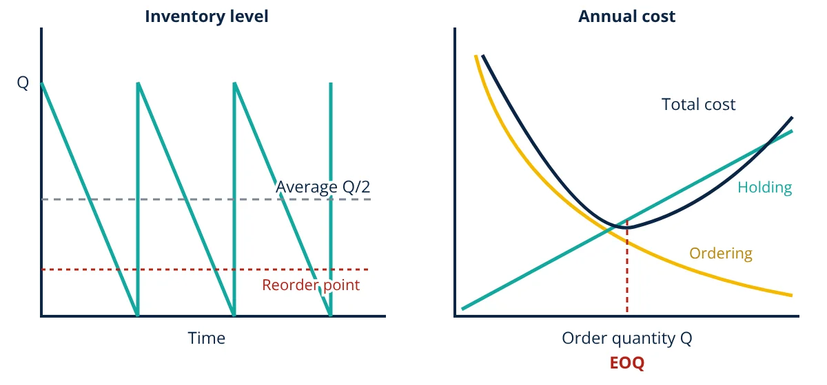
The EOQ (economic order quantity) model finds the order size that minimises the total cost of ordering and holding inventory. Ordering more at once reduces the number of orders but raises average stock and holding cost; ordering less does the opposite. The optimum is EOQ = √(2DS/H), where D is annual demand, S the cost per order (or setup) and H the annual holding cost per unit. At the EOQ, annual ordering cost equals annual holding cost. A reorder point, demand during lead time plus safety stock, tells when to order.
Inventory protects production and customers against delays, but it ties up cash, takes space and risks damage and obsolescence. Ordering too often is also costly, because each order or production setup has fixed administrative, transport or changeover costs. The EOQ model, one of the oldest results in operations management (Harris, 1913), balances these opposing costs.
Assumptions of the basic EOQ model
- Demand is known and constant over time.
- Lead time is known and constant.
- The whole order arrives at once.
- Ordering (or setup) cost per order is fixed regardless of quantity.
- Holding cost is proportional to average inventory.
- No quantity discounts; no stockouts allowed.
These assumptions are simplifications, but the model is robust: total cost changes little for order sizes near the EOQ.
Inventory pattern and costs
With order quantity Q, inventory drops steadily from Q to zero, then a new order arrives. Average inventory is Q/2.
Annual costs as a function of Q:
where D is annual demand (units per year), S the cost per order or setup, and H the holding cost per unit per year. H is often expressed as a percentage i of unit cost C, so H = iC; typical carrying rates are 15 to 30% per year, covering capital, storage, insurance, obsolescence and handling.
Deriving the EOQ
Setting the derivative of TC with respect to Q to zero:
At this quantity, ordering cost equals holding cost, and total cost is TC* = √(2DSH).
Reorder point and safety stock
With daily demand d and lead time L days, the reorder point is:
Safety stock SS protects against variation in demand and lead time. A common formula for variable demand is SS = z σ_d √L, where z is the service level factor (1.65 for about 95%) and σ_d the standard deviation of daily demand.
- Given
- A plant uses 12 000 bearings per year (240 working days). Each order costs 1500 to place and receive. Each bearing costs 400, and the annual holding rate is 20%. Supplier lead time is 10 days. Daily demand has a standard deviation of 12 units; target service level 95% (z = 1.65).
- Find
- EOQ, number of orders per year, total annual ordering and holding cost, safety stock and reorder point.
- Assumptions
- Basic EOQ assumptions; costs in consistent currency units.
- Solution
- H = 0.20 × 400 = 80 per unit per year
EOQ = √(2 × 12 000 × 1500 ÷ 80) = √450 000 = 671 units
Orders per year = 12 000 ÷ 671 ≈ 17.9
Ordering cost = 17.9 × 1500 = 26 830; holding cost = (671 ÷ 2) × 80 = 26 840; total ≈ 53 670
d = 12 000 ÷ 240 = 50 per day; SS = 1.65 × 12 × √10 = 63 units
ROP = 50 × 10 + 63 = 563 units - Answer
- Order about 670 bearings each time, about 18 times a year, when stock falls to about 563 units; annual cost about 53 700
- Limitations
- Real orders may be rounded to pack sizes or adjusted for quantity discounts; demand changes require recalculation.
Extensions of the EOQ model
- Economic production quantity (EPQ): when items are produced gradually at rate p rather than arriving all at once, EPQ = √(2DS ÷ (H(1 − d/p))). S is the machine setup cost.
- Quantity discounts: compare total cost including purchase price at each price break.
- Planned backorders: allow shortages at a cost when customers will wait.
- Periodic review systems: order up to a target level at fixed intervals.
- ABC analysis: apply tight control and EOQ calculations to high value A items, simpler rules to low value C items.
Where EOQ is used
EOQ calculations are common for purchased parts and materials with steady usage, such as fasteners, bearings, packaging, chemicals and spare parts for maintenance stores. In manufacturing, the EPQ version sets batch sizes for parts made on shared machines, where each changeover has a setup cost. Distribution centres use EOQ logic to decide how often to replenish fast moving items from suppliers. ERP systems often include EOQ as one of several lot sizing rules, alongside lot for lot and fixed period ordering.
Steps to apply the EOQ model
- Estimate annual demand from sales forecasts or consumption history.
- Estimate ordering or setup cost: purchasing staff time, transport, receiving, inspection or machine changeover.
- Estimate holding cost: cost of capital plus storage, insurance, handling, obsolescence and damage, usually as a percentage of unit cost.
- Calculate EOQ, then round to practical pack, pallet or container sizes.
- Set safety stock and reorder point based on lead time and demand variation.
- Review parameters regularly, at least yearly or when demand or costs change.
A note on units
Keep units consistent: if demand is annual, holding cost must be per unit per year. If demand is monthly, use a monthly holding cost. Mixing periods is the most common mistake in EOQ calculations and gives answers that are wrong by a factor of √12 or more.
Sensitivity and practical use
Because the total cost curve is flat near its minimum, ordering 20% more or less than the EOQ raises cost by only about 2%. This makes the model useful even with rough estimates. More important is the insight it gives: reducing ordering or setup cost reduces the optimal batch size, which is the logic behind quick changeover and small lot production in lean manufacturing, where excess stock is one of the seven wastes. In MRP systems, EOQ is one of the lot sizing options used in production planning and control.
Frequently asked questions
What does EOQ stand for?
EOQ stands for economic order quantity: the order size that minimises the total annual cost of ordering and holding inventory, given steady demand. The classic formula was published by Ford W. Harris in 1913 and popularised by R. H. Wilson.
Is the EOQ model still useful when demand varies?
The basic model assumes constant demand, but the total cost curve is flat near the optimum, so moderate errors in demand or cost estimates change total cost only slightly. EOQ is therefore a robust starting point. For variable demand, it is combined with safety stock and reorder points, or replaced by dynamic lot sizing in MRP.
How does EOQ relate to lean and just in time?
Lean aims to make small batches economical by cutting setup and ordering costs, for example with quick changeover (SMED) and supplier partnerships. In the EOQ formula, a lower ordering or setup cost directly lowers the optimal order quantity, so lean and EOQ point in the same direction.
References
- F. W. Harris, How Many Parts to Make at Once, Factory, The Magazine of Management, 10(2), 1913
- E. A. Silver, D. F. Pyke and D. J. Thomas, Inventory and Production Management in Supply Chains, 4th ed., CRC Press
- W. J. Stevenson, Operations Management, 14th ed., McGraw-Hill
- S. Chopra and P. Meindl, Supply Chain Management: Strategy, Planning, and Operation, 7th ed., Pearson
Get one engineering email a week
New articles, worked examples and study notes every week. Free, no spam, unsubscribe any time.