PID Controller Explained with Tuning Methods
A PID controller is a feedback controller that computes its output from the error between the setpoint and the measured value using three terms: proportional (present error), integral (accumulated past error) and derivative (rate of change of error). Tuning picks the three gains, by methods such as Ziegler-Nichols or lambda tuning, for fast and stable control.
A PID controller is the most common control algorithm in industry. It runs inside PLCs, DCS controllers, servo drives, temperature controllers and drone flight boards. It measures a process variable, compares it with the setpoint and moves an actuator, such as a valve, heater or motor, to drive the error to zero.
How a PID controller works in a closed loop
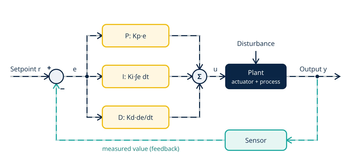
The controller sits in a feedback loop. A sensor measures the output y of the plant (the actuator plus the process). The summing junction subtracts this measured value from the setpoint r to form the error e = r - y. The P, I and D terms each act on the error, and their sum is the controller output u that drives the plant. Disturbances such as a change in load push y away from r, and the loop corrects them.
The three terms of a PID controller
The proportional (P) term changes the output in proportion to the present error: u = Kp·e. A larger Kp gives a faster response, but too much gain causes overshoot and oscillation. On a plant without its own integrating action, P alone leaves a steady-state error (offset), because some error is needed to hold a non-zero output.
The integral (I) term adds up the error over time. As long as any error remains, the integral keeps changing the output, so it removes the steady-state offset. It also adds phase lag, so too much integral action makes the loop slower to settle and more oscillatory.
The derivative (D) term responds to how fast the error is changing. It anticipates where the error is heading and brakes the output, which adds damping and reduces overshoot. Because it amplifies high frequency noise, practical controllers filter the derivative and often apply it to the measured value rather than the error, which avoids a large “derivative kick” when the setpoint is stepped.
| Increase in | Rise time | Overshoot | Steady-state error | Main side effect |
|---|---|---|---|---|
| Kp | Shorter | Larger | Smaller, not zero | Oscillation at high gain |
| Ki (shorter Ti) | Shorter | Larger | Removed | Slower settling, windup |
| Kd (longer Td) | Small change | Smaller | No direct effect | Noise amplification |
The PID equation
The standard (ideal or ISA) form of the PID controller is:
Here Ti is the integral time and Td the derivative time, both in seconds. The same controller in parallel form uses separate gains:
In the Laplace domain the standard form has the transfer function:
Controller manufacturers use different forms and units (gain or proportional band, repeats per minute or minutes per repeat), so always check which form a controller uses before copying tuning values between them.
PID controller tuning methods
Tuning means choosing Kp, Ti and Td for a particular plant. You want a response that is fast, has acceptable overshoot, rejects disturbances and stays stable when the plant changes a little.
Ziegler-Nichols ultimate gain method
Ziegler and Nichols published two rules in 1942. In the closed loop (ultimate gain) method:
- Put the controller in P only mode (integral off, derivative zero).
- Raise Kp slowly until the measured value oscillates with constant amplitude.
- Record this ultimate gain Ku and the period of oscillation Pu.
- Calculate the settings from the table below.
| Controller | Kp | Ti | Td |
|---|---|---|---|
| P | 0.5 Ku | not used | not used |
| PI | 0.45 Ku | Pu / 1.2 | not used |
| PID | 0.6 Ku | Pu / 2 | Pu / 8 |
The test pushes the loop to the edge of stability, so it is not acceptable on every plant.
Ziegler-Nichols step response method
In the open loop method, the controller is put in manual and the output is stepped. The response is fitted with a dead time L and a slope R, and a = R·L, normalised by the size of the output step. The PID settings are Kp = 1.2/a, Ti = 2L and Td = L/2 (for PI: Kp = 0.9/a and Ti = 3L). Both Ziegler-Nichols rules aim for a quarter amplitude decay ratio, which is fast but oscillatory.
Lambda tuning
For a process modelled as first order plus dead time, with process gain K, time constant T and dead time L, lambda tuning sets Ti = T and Kp = T / (K(λ + L)). The engineer chooses the desired closed loop time constant λ: a larger λ gives a slower, smoother and more robust loop. It is widely used on process plants because it gives no overshoot to setpoint changes and predictable behaviour.
Other methods include Cohen-Coon, internal model control (IMC) rules and the relay autotuners built into many modern controllers.
- Given
- A temperature loop is tested with the ultimate gain method. Sustained oscillation starts at Ku = 4.0 %/°C with a period Pu = 20 s. Later, at one instant, the error is 2 °C, the integral of error is 10 °C·s and the error is falling at 0.5 °C/s.
- Find
- (a) Ziegler-Nichols PID settings Kp, Ti and Td; (b) the equivalent parallel gains Ki and Kd; (c) the controller output at that instant.
- Assumptions
- Standard (ISA) PID form; output in percent of span; no output bias; no derivative filter or saturation.
- Solution
- (a) Kp = 0.6 × 4.0 = 2.4 %/°C; Ti = 20 / 2 = 10 s; Td = 20 / 8 = 2.5 s
(b) Ki = Kp / Ti = 2.4 / 10 = 0.24 %/(°C·s); Kd = Kp × Td = 2.4 × 2.5 = 6.0 %·s/°C
(c) P term = 2.4 × 2 = 4.8 %; I term = 0.24 × 10 = 2.4 %; D term = 6.0 × (-0.5) = -3.0 %; u = 4.8 + 2.4 - 3.0 = 4.2 % - Answer
- Kp = 2.4 %/°C, Ti = 10 s, Td = 2.5 s (Ki = 0.24 %/(°C·s), Kd = 6.0 %·s/°C); controller output 4.2 %
- Limitations
- Ziegler-Nichols settings are a starting point aimed at quarter amplitude decay; the loop is usually detuned after testing. A real controller also adds an output bias, a derivative filter and output limits with anti-windup.
In part (c) the D term is negative because the error is already shrinking, so it holds the output back. That is the damping that limits overshoot.
Practical issues in PID control
- Integral windup: when the actuator saturates, the integral keeps growing and later causes a large overshoot. Clamping (conditional integration) or back-calculation stops it.
- Derivative noise: a first order filter on the derivative term limits the gain at high frequency. Many loops simply run as PI.
- Bumpless transfer: switching from manual to automatic must not cause a sudden output jump, so the controller initialises its integral to the current output.
- Sampling: digital controllers in a PLC or DCS run the algorithm at a fixed scan time, which must be short compared with the process dynamics.
- Direct or reverse action: the controller action must match the plant. For example, a cooling valve must open as temperature rises.
PID loops appear at every level of automation: nested current, velocity and position loops in servo drives, attitude control in a quadcopter, process loops in a DCS and temperature and humidity control in greenhouses. The sensor, controller and actuator chain is covered in mechatronic system elements.
Key formulas for PID controller
| Quantity | Formula | Symbols and units |
|---|---|---|
| Error | e = r - y | r setpoint, y measured value, same units |
| PID output (standard form) | u = Kp[e + (1/Ti)∫e dt + Td de/dt] | Kp gain, Ti and Td in s |
| Parallel gains | Ki = Kp/Ti, Kd = Kp·Td | Ki in gain per s, Kd in gain·s |
| Transfer function | C(s) = Kp(1 + 1/(Ti s) + Td s) | s Laplace variable |
| Ziegler-Nichols PID (ultimate gain) | Kp = 0.6Ku, Ti = Pu/2, Td = Pu/8 | Ku ultimate gain, Pu period in s |
| Ziegler-Nichols PI (ultimate gain) | Kp = 0.45Ku, Ti = Pu/1.2 | as above |
| Lambda tuning (PI) | Kp = T/(K(λ + L)), Ti = T | K process gain, T time constant, L dead time, λ closed loop time constant |
PID controller interview and viva questions
- Why does a P only controller leave a steady-state error? On a plant without integrating action, a non-zero output is needed to hold the process at the setpoint, and a proportional controller can only produce that output from a non-zero error.
- What does the integral term add, and what is its drawback? It removes steady-state error by accumulating error over time, but it adds phase lag, which makes the loop more oscillatory and can cause integral windup when the actuator saturates.
- Why is derivative action often applied to the measured value instead of the error? A setpoint step makes the error jump instantly, so derivative on error gives a large output spike (derivative kick); using the measured value avoids it.
- How do you find Ku and Pu in the Ziegler-Nichols ultimate gain method? With integral and derivative off, raise the proportional gain until the loop oscillates with constant amplitude; that gain is Ku and the oscillation period is Pu.
- What is the relation between the standard and parallel PID forms? The parallel gains are Ki = Kp/Ti and Kd = Kp·Td, so the same controller can be written either way, but tuning values must be converted before moving them between forms.
Frequently asked questions
Why do most process loops use PI instead of full PID control?
Many process loops, such as flow and pressure, respond quickly and carry noisy measurements. Derivative action amplifies that noise and adds little benefit, so a PI controller gives zero steady-state error with less actuator wear. Derivative is mostly added on slow loops such as temperature.
What is integral windup?
When the actuator saturates, for example a valve fully open, the error stays large and the integral term keeps growing. When the error finally reverses, the oversized integral holds the output at its limit and causes a large overshoot. Anti-windup methods such as clamping or back-calculation stop the integral from growing while the output is saturated.
Is Ziegler-Nichols tuning good enough for a real plant?
It gives a quick starting point, but its settings aim for quarter amplitude decay, which is oscillatory and has poor robustness for many loops. Engineers usually detune the gains afterwards or use methods such as lambda tuning that trade speed for a smoother, more robust response.
References
- K. J. Åström and T. Hägglund, Advanced PID Control, ISA, 2006
- K. Ogata, Modern Control Engineering, 5th ed., Prentice Hall, 2010
- J. G. Ziegler and N. B. Nichols, Optimum Settings for Automatic Controllers, Transactions of the ASME, vol. 64, pp. 759 to 768, 1942
- D. E. Seborg, T. F. Edgar, D. A. Mellichamp and F. J. Doyle, Process Dynamics and Control, 4th ed., Wiley, 2016
- N. S. Nise, Control Systems Engineering, 7th ed., Wiley, 2015
Get one engineering email a week
New articles, worked examples and study notes every week. Free, no spam, unsubscribe any time.