Finite Element Analysis (FEA): Basic Steps Explained
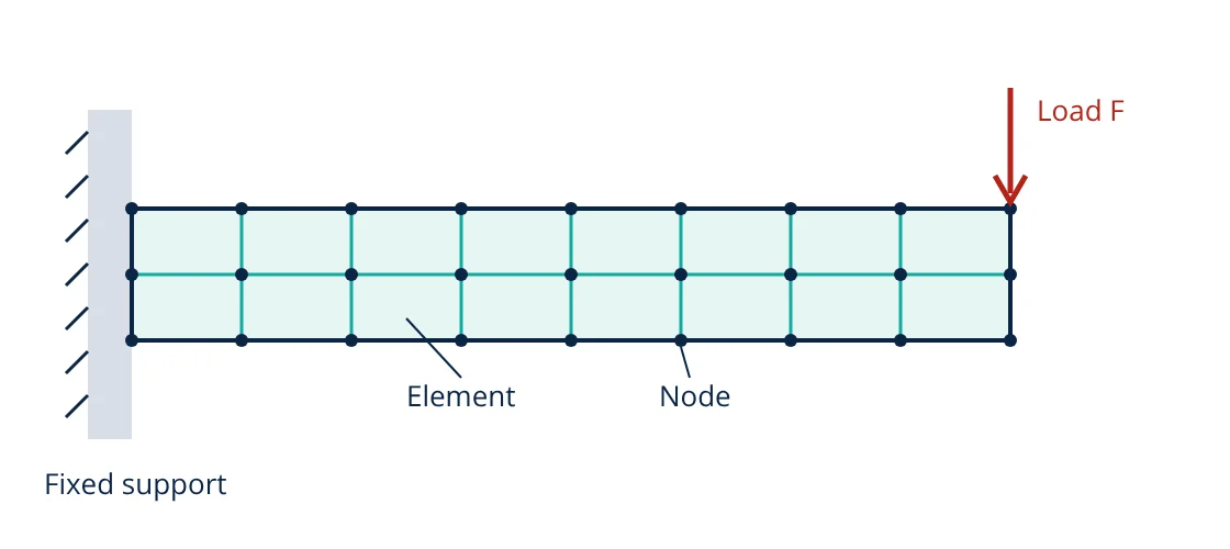
Finite element analysis (FEA) predicts how a part behaves under load by dividing it into many small, simple pieces called elements, connected at points called nodes. Simple equations are written for each element, assembled into one large system and solved by computer for the unknown displacements. Strains and stresses then follow. Every analysis has three stages: pre-processing (model, material, mesh, loads, supports), solution and post-processing (results and checks).
Most real parts have shapes too complex for textbook formulas. Finite element analysis turns such a problem into a large but straightforward set of algebraic equations that a computer can solve. It is used for stress and deflection, heat transfer, vibration, fluid flow and electromagnetics. This article explains the basic idea and the steps every engineer should follow, so that results can be trusted rather than just admired.
The basic idea of finite element analysis
A continuous body has infinitely many points, so its exact deformation is hard to find. FEA approximates it with a finite number of nodes. Within each element, displacement is assumed to vary in a simple way (linearly or quadratically) between the nodes, through shape functions. The problem then reduces to finding the displacements at the nodes.
For linear static problems, each element gives a stiffness relation between its nodal forces and nodal displacements. These are assembled into a global system:
K is the global stiffness matrix, u the vector of unknown nodal displacements and F the vector of applied nodal forces. It is the same idea as a spring, F = k x, scaled up to thousands or millions of equations. After the boundary conditions are applied, the solver finds u. Strains come from the derivatives of the displacements, and stresses from the material law, which for linear elastic materials is Hooke’s law; see stress and strain.
Steps of a finite element analysis
1. Define the problem
Decide what question the analysis must answer: peak stress, deflection, natural frequency, temperature or fatigue life. Identify the loads, the operating conditions and the acceptance criteria, such as an allowable stress based on the factor of safety. Estimate the expected answer with a hand calculation before starting.
2. Pre-processing
- Geometry: import from CAD and simplify. Remove small features that do not affect the result (logos, small holes far from critical areas), but keep fillets and holes in high stress regions. Use symmetry to reduce model size.
- Element type: beams and shells for slender or thin parts; solid tetrahedral or hexahedral elements for chunky parts. Second order (quadratic) elements are usually more accurate for stress.
- Material properties: Young’s modulus, Poisson’s ratio and density for linear static work; plasticity, temperature dependence or anisotropy where needed.
- Mesh: generate elements and refine them where stress gradients are high.
- Boundary conditions: supports and constraints that represent how the part is really held. This is the most common source of error.
- Loads: forces, pressures, temperatures, accelerations, bolt preloads. Spread point loads over realistic areas.
3. Solution
The software assembles and solves the equations. Linear static problems solve in one step. Nonlinear problems (large deflection, plasticity, contact) are solved in increments with iterations. Dynamic analyses find natural frequencies (modal) or the response over time. Thermal analyses solve for temperature using the modes of heat transfer as boundary conditions; the temperature field can then be passed to a stress analysis.
4. Post-processing
Review deformed shape, displacement, stress and reaction forces. For ductile metals the von Mises (equivalent) stress is compared with yield strength. Do not stop at a colourful contour plot.
5. Verify and validate
- Sanity checks: does the deformed shape look physically right? Do reaction forces balance the applied loads?
- Mesh convergence: refine the mesh and confirm the result of interest changes by only a few percent.
- Hand calculation: compare with a simple formula for a simplified version of the problem.
- Test data: strain gauge or deflection measurements on a prototype validate the model.
- Given
- An FEA model of a steel cantilever, length 1 m, rectangular section 50 mm wide × 100 mm deep, E = 200 GPa, loaded by 1 kN at the free end, reports a tip deflection of 0.41 mm and a peak bending stress of 12.1 MPa away from the support.
- Find
- Hand calculation values to check the model.
- Assumptions
- Euler-Bernoulli beam theory, linear elastic material, shear deflection neglected, ideal fixed support.
- Solution
- I = b h³ / 12 = 50 × 100³ / 12 = 4.167 × 10⁶ mm⁴
δ = F L³ / (3 E I) = 1000 × 1000³ / (3 × 200,000 × 4.167 × 10⁶) = 0.40 mm
M = F L = 1000 × 1000 = 10⁶ N·mm; σ = M (h/2) / I = 10⁶ × 50 / 4.167 × 10⁶ = 12.0 MPa - Answer
- Hand values 0.40 mm and 12.0 MPa agree with the FEA within about 3 percent, so the model setup is credible
- Limitations
- The small extra FEA deflection is expected from shear deformation, which beam theory ignores. Stress right at the fixed edge is affected by the idealised support and should not be read directly.
Common mistakes in FEA
- Wrong boundary conditions: fully fixing a face that really flexes, or under-constraining so the model can move freely.
- Trusting singularities: sharp corners and point loads give stresses that grow without limit as the mesh is refined.
- Wrong units: mixing mm with m or MPa with Pa. Check the unit system before solving.
- Ignoring nonlinearity: contact, large deflection and yielding need nonlinear analysis.
- No convergence study: a coarse mesh usually under-predicts peak stress.
Applications
FEA is used across engineering: machine frames and shafts, pressure vessels, pump casings like that of a centrifugal pump, heat exchangers, vehicle crash structures, PCB thermal design and civil structures. It pairs with computational fluid dynamics, which applies similar numerical ideas to fluid flow governed by the same conservation laws behind the Bernoulli equation.
Related reading
Frequently asked questions
What is the difference between FEA and FEM?
The finite element method (FEM) is the mathematical technique of dividing a domain into elements and solving approximate equations. Finite element analysis (FEA) is the engineering use of that method, usually through software, to predict stress, deflection, temperature or other responses.
How fine should an FEA mesh be?
Fine enough that the result of interest stops changing significantly when the mesh is refined further. This is checked with a mesh convergence study: refine the mesh in the critical region two or three times and compare the peak values.
Why does my FEA show very high stress at a sharp corner or point load?
A perfectly sharp re-entrant corner or a load applied at a single node is a mathematical singularity, where theoretical stress is infinite. The reported value keeps rising as the mesh is refined. Model a real fillet radius and spread loads over a realistic area, or judge the result away from the singular point.
Can FEA replace physical testing?
It reduces the number of prototypes and tests but does not remove them. Simulations rest on assumptions about loads, materials and boundary conditions, so critical designs are still validated by test, and test data is used to calibrate models.
References
- R. D. Cook, D. S. Malkus, M. E. Plesha and R. J. Witt, Concepts and Applications of Finite Element Analysis, 4th ed., Wiley
- D. L. Logan, A First Course in the Finite Element Method, 6th ed., Cengage
- O. C. Zienkiewicz, R. L. Taylor and J. Z. Zhu, The Finite Element Method: Its Basis and Fundamentals, 7th ed., Butterworth-Heinemann
- NAFEMS, How to Plan a Finite Element Analysis, NAFEMS
Get one engineering email a week
New articles, worked examples and study notes every week. Free, no spam, unsubscribe any time.