Thevenin's Theorem: Steps and Solved Examples
Thevenin’s theorem states that any linear two-terminal circuit, however complex, can be replaced at its terminals by a single voltage source Vth in series with a single resistance Rth. Vth is the open-circuit voltage at the terminals, and Rth is the resistance seen at the terminals with all independent sources turned off.
Thevenin’s theorem is one of the most useful tools in circuit analysis. It lets an engineer collapse a large network into a two-element model and then study what happens when only the load changes. This guide explains the theorem, gives the step by step method, covers circuits with dependent sources, links Thevenin and Norton forms, and solves a complete example including maximum power transfer.
What Thevenin’s theorem says
The French engineer Léon Charles Thévenin published the theorem in 1883. It applies to any circuit made of linear elements (resistors, inductors, capacitors, linear dependent sources) and independent sources. Looking into two terminals A and B, the whole circuit behaves exactly like:
- an ideal voltage source Vth, equal to the voltage across A and B when nothing is connected, in series with
- a resistance Rth, equal to the resistance measured across A and B with independent sources deactivated.
“Behaves exactly like” means that for any load connected across A and B, the load voltage and current are the same in the original circuit and in the equivalent. What happens inside the original circuit, such as the power lost in its internal resistors, is not represented by the equivalent.
The load current follows directly from the model:
Steps to apply Thevenin’s theorem
- Identify the load. Choose the element or branch you want to study and remove it. Mark the two terminals A and B where it was connected.
- Find Vth. Calculate the open-circuit voltage between A and B using any method: voltage divider, nodal analysis, mesh analysis or superposition. The basic tools are covered in Ohm’s law and Kirchhoff’s laws.
- Find Rth. Turn off every independent source: replace voltage sources with short circuits and current sources with open circuits. Then find the equivalent resistance between A and B by series and parallel reduction. Where resistors form a bridge, a star delta transformation may be needed.
- Draw the equivalent. Place Vth in series with Rth, with the polarity that gives the open-circuit voltage you found.
- Reconnect the load. Calculate the load current and voltage from the simple series circuit.
An alternative to step 3 is to find the short-circuit current Isc between A and B. Then Rth = Vth / Isc. This is also how an equivalent is found from measurements on real equipment: measure the open-circuit voltage, then the current into a known load, and solve for Rth.
Circuits with dependent sources
Dependent (controlled) sources must not be switched off, because their value depends on a voltage or current elsewhere in the circuit. Two methods are used:
- Test source method: turn off independent sources only, apply a test voltage Vt across A and B, find the current It it delivers, and take Rth = Vt / It.
- Open circuit and short circuit method: find Vth and Isc with all sources active, then divide.
With dependent sources Rth can even come out negative, which indicates that the circuit can supply energy, as in an amplifier model.
Thevenin and Norton equivalents
Norton’s theorem gives the dual result: the same terminals can be modelled by a current source IN in parallel with a resistance RN. The two forms are related by source transformation:
Use whichever form makes the next step easier. A Thevenin model suits loads added in series; a Norton model suits loads added in parallel.
Maximum power transfer
For a source with a fixed Thevenin resistance, the power delivered to a resistive load is greatest when RL = Rth. The maximum power is then:
At this point the efficiency is only 50 percent, because equal power is lost in Rth. Power systems therefore do not operate at matched conditions; they keep the source resistance much smaller than the load to achieve high efficiency. Matching is used in communication and signal circuits, where getting the most power to a load matters more than efficiency. In AC circuits the condition becomes a load impedance equal to the complex conjugate of the source impedance.
- Given
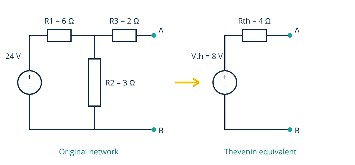
- A 24 V DC source feeds R1 = 6 Ω in series, then R2 = 3 Ω connected across the circuit, then R3 = 2 Ω in series to terminals A and B, as in the figure. A load RL = 4 Ω is connected across A and B.
- Find
- The Thevenin equivalent at A and B, the load current, and the load power. Check whether this load receives maximum power.
- Assumptions
- Ideal source with zero internal resistance, linear resistors, steady DC conditions.
- Solution
- Remove RL. With A and B open, no current flows in R3, so Vth equals the voltage across R2.
Vth = 24 × 3 / (6 + 3) = 8 V
Short the 24 V source. R1 and R2 are now in parallel, in series with R3.
Rth = (6 × 3) / (6 + 3) + 2 = 2 + 2 = 4 Ω
IL = 8 / (4 + 4) = 1.0 A
PL = 1.0² × 4 = 4.0 W
Pmax = 8² / (4 × 4) = 4.0 W - Answer
- Vth = 8 V, Rth = 4 Ω, load current 1.0 A, load power 4.0 W. Since RL = Rth, this is the maximum power the network can deliver.
- Limitations
- The equivalent predicts only terminal quantities. The power lost inside R1, R2 and R3 is not 4 W and must be found from the original circuit. A real source has internal resistance, which would add to R1.
To check the result, solve the original circuit directly with the 4 Ω load. R3 plus RL is 6 Ω, which in parallel with R2 gives 2 Ω. The total resistance is 8 Ω, so the source current is 3 A and the voltage across R2 is 6 V. The load branch current is 6 / 6 = 1 A, matching the Thevenin result.
Where Thevenin’s theorem is used
- Load studies: finding the current in one branch for many values of load without re-solving the whole network.
- Fault calculations: the Thevenin impedance at a bus in a power system sets the short circuit current at that point.
- Electronics: modelling a sensor, signal source or bias network as a source with an output resistance, which shows how much the reading drops when a meter or amplifier input loads it.
- Instrumentation: checking that a transmitter loop or bridge output is not pulled down by the input resistance of the measuring device.
Common mistakes
- Leaving the load connected while finding Vth.
- Opening a voltage source instead of shorting it when finding Rth.
- Switching off dependent sources.
- Using the equivalent to calculate power inside the original network.
- Getting the polarity of Vth wrong, which reverses the load current.
Related reading
Frequently asked questions
Can Thevenin's theorem be used for AC circuits?
Yes. For a linear AC circuit at a single frequency, the same steps are carried out with phasors and impedances. The result is a Thevenin voltage phasor in series with a Thevenin impedance, which can include resistance and reactance.
Why are voltage sources shorted when finding Rth?
Finding Rth means looking at the circuit with all independent sources set to zero. A voltage source set to zero volts behaves like a short circuit, and a current source set to zero amperes behaves like an open circuit. Dependent sources are left in place.
Does Thevenin's theorem work for non-linear circuits?
No. The theorem relies on superposition, which holds only for linear elements. A circuit containing diodes or transistors can be replaced by a Thevenin equivalent only around a fixed operating point, using a linearized small signal model.
References
- C. K. Alexander and M. N. O. Sadiku, Fundamentals of Electric Circuits, 7th ed., McGraw-Hill
- W. H. Hayt, J. E. Kemmerly and J. D. Phillips, Engineering Circuit Analysis, 9th ed., McGraw-Hill
- J. W. Nilsson and S. A. Riedel, Electric Circuits, 11th ed., Pearson
- R. L. Boylestad, Introductory Circuit Analysis, 13th ed., Pearson
Get one engineering email a week
New articles, worked examples and study notes every week. Free, no spam, unsubscribe any time.