Big O Notation Explained with Examples
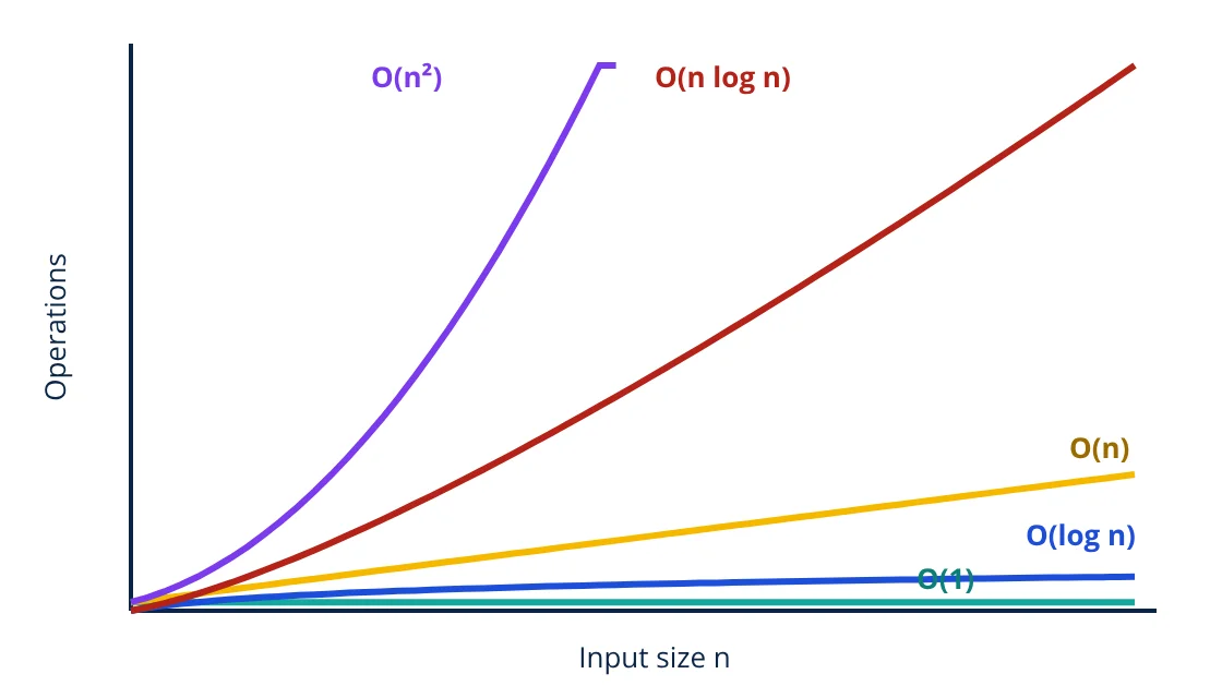
Big O notation describes how the running time or memory of an algorithm grows as the input size n grows, ignoring constant factors and smaller terms. O(1) means constant time, O(log n) logarithmic, O(n) linear, O(n log n) typical of efficient sorting, O(n²) quadratic and O(2ⁿ) exponential. It lets engineers compare algorithms independently of hardware and predict how a program will scale.
Two programs that solve the same problem may both finish instantly on 100 items, yet one takes seconds and the other hours on 10 million. Big O notation explains why. It is the standard language for discussing algorithm efficiency in textbooks, documentation and technical interviews.
What Big O notation measures
Big O counts how the number of basic steps (comparisons, assignments, arithmetic operations) grows with the input size n, for large n. Formally, a function f(n) is O(g(n)) if there are positive constants c and n₀ such that:
In words, beyond some input size, f grows no faster than a constant multiple of g. That is why constants and lower order terms disappear: 3n² + 5n + 20 is O(n²), because for large n the n² term dominates.
Related notations are Big Omega (Ω, a lower bound) and Big Theta (Θ, a tight bound). Analyses also distinguish the worst case, average case and best case. Big O of the worst case is the most commonly quoted figure because it gives a guarantee.
Common complexity classes
| Big O | Name | Example |
|---|---|---|
| O(1) | Constant | Reading an array element by index; hash table lookup on average |
| O(log n) | Logarithmic | Binary search in a sorted array; balanced tree search |
| O(n) | Linear | Scanning a list for a value; summing an array |
| O(n log n) | Linearithmic | Merge sort, heapsort; average quicksort |
| O(n²) | Quadratic | Comparing every pair; bubble and insertion sort in the worst case |
| O(n³) | Cubic | Naive matrix multiplication |
| O(2ⁿ) | Exponential | Trying every subset of n items |
| O(n!) | Factorial | Trying every ordering, as in brute force travelling salesman |
How to find the Big O of code
- Count loops. A single loop over n items is O(n). Two nested loops over n are O(n²). A loop that halves the problem each step is O(log n).
- Add sequential parts, then keep the largest. O(n) + O(n²) = O(n²).
- Multiply nested parts. An O(log n) operation inside an O(n) loop gives O(n log n).
- Drop constants. O(2n) is O(n); O(n/2) is O(n).
- Use different letters for different inputs. Looping over a list of length a and another of length b nested gives O(a × b), not O(n²).
- Recursion: set up a recurrence. Merge sort satisfies T(n) = 2T(n/2) + O(n), which solves to O(n log n).
def has_duplicate_pairwise(items):      # O(n^2): compares every pair
    for i in range(len(items)):
        for j in range(i + 1, len(items)):
            if items[i] == items[j]:
                return True
    return False

def has_duplicate_set(items):           # O(n) on average: one pass with a hash set
    seen = set()
    for x in items:
        if x in seen:
            return True
        seen.add(x)
return False- Given
- A sorted list of one million items and a computer that performs about one comparison per nanosecond.
- Find
- Worst case comparisons and time for linear search, binary search and an O(n²) pairwise check.
- Assumptions
- Each comparison costs the same; other overheads ignored.
- Solution
- Linear search: up to 10⁶ comparisons, about 1 ms
Binary search: about log₂(10⁶) ≈ 20 comparisons, about 20 ns
Pairwise check: n(n − 1)/2 ≈ 5 × 10¹¹ comparisons, about 500 s - Answer
- About 1 ms, 20 ns and over 8 minutes respectively: the growth rate, not the hardware, decides feasibility
- Limitations
- Real timings depend on memory access, caches and language overheads, but the ratios between growth classes stay huge.
Big O of common data structure operations
| Structure | Access | Search | Insert | Delete |
|---|---|---|---|---|
| Array | O(1) | O(n) | O(n) | O(n) |
| Sorted array | O(1) | O(log n) | O(n) | O(n) |
| Linked list | O(n) | O(n) | O(1) at known node | O(1) at known node |
| Hash table (average) | Not applicable | O(1) | O(1) | O(1) |
| Balanced binary search tree | O(log n) | O(log n) | O(log n) | O(log n) |
Knowing these costs lets you choose a structure by looking at which operations your program performs most often.
Space complexity
Big O also describes memory. The set based duplicate check above uses O(n) extra space; the pairwise check uses O(1) extra space. Many design decisions trade time for space, for example caching results (memoisation) or building an index. The memory overhead of arrays vs linked lists is a practical example.
Amortised complexity
Some operations are usually cheap but occasionally expensive. Appending to a dynamic array is O(1) most of the time, but O(n) when the array must grow and copy. Because growth doubles the capacity, the total cost of n appends is O(n), so each append is amortised O(1).
Common mistakes
- Treating Big O as exact running time; it hides constants that matter for small n.
- Forgetting hidden loops inside library calls, such as searching a list with the in operator inside another loop.
- Ignoring the cost of data movement and memory access patterns.
- Quoting the average case when inputs may be adversarial; quicksort is O(n²) in the worst case.
Big O thinking applies across computer science: from choosing data structures to designing database queries, where good normalization and indexes avoid scanning whole tables. Language implementation affects only constant factors, as explained in compiled vs interpreted languages, while the choice of algorithm changes the growth rate itself. Writing unit tests for edge cases helps confirm that a faster algorithm still gives correct results.
Frequently asked questions
What is the difference between Big O, Big Omega and Big Theta?
Big O gives an upper bound on growth, Big Omega a lower bound and Big Theta a tight bound, meaning both. In everyday use, people often say Big O when they mean the tight bound of the worst case, but formally O(n²) is also a true (if loose) upper bound for an O(n) algorithm.
Is O(n log n) better than O(n)?
No. For large n, n log n grows faster than n, so an O(n) algorithm scales better. O(n log n) is, however, the best possible worst case for sorting by comparisons, which is why efficient sorts such as merge sort and heapsort have that complexity.
Does Big O tell me which program is faster?
Not exactly. It describes how running time grows with input size and ignores constant factors and lower order terms. For small inputs, or when constants differ greatly, an algorithm with worse Big O can run faster. Big O guides design; profiling decides real performance.
References
- T. H. Cormen, C. E. Leiserson, R. L. Rivest and C. Stein, Introduction to Algorithms, 4th ed., MIT Press
- D. E. Knuth, Big Omicron and Big Omega and Big Theta, SIGACT News, 1976
- J. Kleinberg and É. Tardos, Algorithm Design, Pearson
Get one engineering email a week
New articles, worked examples and study notes every week. Free, no spam, unsubscribe any time.