Tokenization and Embeddings in NLP Explained
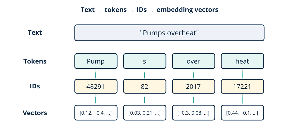
Tokenization and embeddings are the first two steps of nearly every NLP system. Tokenization splits text into small units called tokens (words, characters or, most often today, subwords) and maps each to an integer ID. Embeddings turn each token ID into a dense vector of numbers, learned so that tokens with similar meanings have similar vectors. Neural networks then process these vectors instead of raw text.
Computers cannot read words; they work with numbers. Natural language processing (NLP) therefore needs a reliable way to convert text into numbers that keep its meaning. Tokenization and embeddings do exactly that, and they sit underneath search engines, chatbots, translation and large language models.
What is tokenization?
Tokenization breaks a string of text into a sequence of tokens from a fixed vocabulary. Each token in the vocabulary has a unique ID. There are three main approaches.
Word tokenization
Split on spaces and punctuation: “The pump failed.” becomes [“The”, “pump”, “failed”, ”.”]. It is simple and readable, but the vocabulary becomes huge, and any word not seen during training (an out of vocabulary word) becomes an unknown token.
Character tokenization
Every character is a token. The vocabulary is tiny and nothing is ever unknown, but sequences become very long and individual characters carry little meaning, which makes learning harder and slower.
Subword tokenization
The standard for modern models. Common words stay whole, and rare words are split into meaningful pieces. “unbelievably” might become [“un”, “believ”, “ably”]. Main algorithms:
- Byte Pair Encoding (BPE): start from characters (or bytes) and repeatedly merge the most frequent adjacent pair into a new token until the vocabulary reaches the target size. Used by GPT models.
- WordPiece: similar, but merges pairs that most increase the likelihood of the training data. Used by BERT.
- Unigram and SentencePiece: treat text as a raw stream including spaces, which works well for languages without spaces such as Japanese and Chinese.
Tokenizers also add special tokens that mark the start and end of sequences, padding, or separators between sentences.
What are embeddings?
Token IDs are only labels. ID 48291 is not “bigger” or “closer” to anything than ID 82; the numbers carry no meaning. A model needs a representation in which related words are near each other, so that what it learns about one word transfers to similar words.
The simplest numeric form of a token is a one-hot vector: a vector as long as the vocabulary, with a 1 at the token’s ID and 0 everywhere else. It is huge, sparse and carries no meaning; every pair of words is equally different.
An embedding replaces this with a short, dense vector, typically 100 to a few thousand numbers. The embedding layer is simply a matrix with one row per token; looking up a token ID returns its row. The values are learned during training so that the geometry of the vectors reflects meaning: “pump” and “compressor” end up close together, far from “banana”.
Static embeddings: Word2Vec and GloVe
Word2Vec (Mikolov and colleagues, 2013) learns vectors by predicting a word from its neighbours (CBOW) or neighbours from a word (skip-gram). The idea, from linguistics, is that words used in similar contexts have similar meanings. GloVe learns vectors from global word co-occurrence counts. These embeddings show famous patterns, such as the vector “king” − “man” + “woman” landing near “queen”.
Their limitation is one vector per word, whatever the context.
Contextual embeddings
Transformer models such as BERT and GPT start from a token embedding, add position information, then pass the sequence through attention layers. The output vector for each token depends on all the surrounding tokens, so “bank” in “river bank” and “bank account” gets different vectors. These contextual embeddings are why modern NLP understands meaning so much better than earlier methods.
Measuring similarity
The closeness of two embedding vectors a and b is usually measured by cosine similarity:
A value near 1 means very similar direction (similar meaning), near 0 means unrelated, and negative means opposite.
- Given
- Three toy 3-dimensional embeddings: pump = (0.8, 0.5, 0.1), compressor = (0.7, 0.6, 0.2), banana = (0.1, 0.2, 0.9).
- Find
- Cosine similarity of pump with compressor and of pump with banana.
- Assumptions
- Toy values for illustration; real embeddings have hundreds of dimensions.
- Solution
- |pump| = √(0.64 + 0.25 + 0.01) = √0.90 = 0.949
|compressor| = √(0.49 + 0.36 + 0.04) = √0.89 = 0.943
|banana| = √(0.01 + 0.04 + 0.81) = √0.86 = 0.927
pump · compressor = 0.56 + 0.30 + 0.02 = 0.88; cos = 0.88 ÷ (0.949 × 0.943) = 0.98
pump · banana = 0.08 + 0.10 + 0.09 = 0.27; cos = 0.27 ÷ (0.949 × 0.927) = 0.31 - Answer
- pump and compressor: 0.98 (very similar); pump and banana: 0.31 (unrelated)
- Limitations
- Similarity reflects patterns in the training text, including its biases, not verified facts.
Where tokenization and embeddings are used
- Semantic search: embed documents and queries, then return the documents with the highest cosine similarity, even when they share no exact words.
- Retrieval augmented generation (RAG): fetch relevant passages by embedding similarity and give them to a language model as context.
- Text classification: sentiment, ticket routing, fault report categorisation.
- Clustering: group similar maintenance logs or customer feedback, an unsupervised learning task.
- Language models: every neural network for language starts with an embedding layer.
Practical tips
- Always use the same tokenizer the model was trained with; a mismatch produces garbage.
- Count tokens, not words, when working with model context limits and API costs.
- Domain jargon, part numbers and tag names often split into many tokens; check how your text tokenizes.
- Watch for multilingual text: languages other than English often need more tokens per word, which affects cost and context length.
- Normalise text consistently (case, Unicode, whitespace) before tokenizing for classical models.
- For search, choose an embedding model trained for retrieval, and store vectors in a vector database or index.
Tokenization and embeddings are where language becomes mathematics. Understanding them makes the behaviour of modern language models, including their limits, much easier to reason about.
Frequently asked questions
Why do language models use subword tokens instead of whole words?
A whole word vocabulary would need millions of entries and still fail on new words, typos and names. Subword methods such as Byte Pair Encoding keep common words as single tokens and split rare words into smaller known pieces, so any text can be represented with a vocabulary of around 30 000 to 200 000 tokens.
How many tokens is a word?
For English text with modern tokenizers, a rough rule is about 0.75 words per token, or about 4 characters per token. Common short words are one token, while long, rare or technical words may be several. Other languages and code can use more tokens per word.
What is the difference between Word2Vec and contextual embeddings?
Word2Vec gives each word a single fixed vector, so 'bank' has the same vector in 'river bank' and 'bank loan'. Contextual embeddings from transformer models such as BERT compute a different vector for each occurrence based on the surrounding words, so the two meanings of 'bank' get different vectors.
References
- D. Jurafsky and J. H. Martin, Speech and Language Processing, 3rd ed. draft, Stanford University
- T. Mikolov et al., Efficient Estimation of Word Representations in Vector Space, 2013
- R. Sennrich, B. Haddow and A. Birch, Neural Machine Translation of Rare Words with Subword Units, ACL, 2016
- J. Devlin et al., BERT: Pre-training of Deep Bidirectional Transformers for Language Understanding, NAACL, 2019
Get one engineering email a week
New articles, worked examples and study notes every week. Free, no spam, unsubscribe any time.