How Neural Networks Work: Neurons, Layers and Training
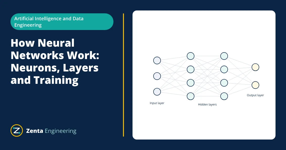
How neural networks work: an artificial neural network is layers of simple neurons. Each neuron multiplies its inputs by weights, adds a bias and applies a non-linear activation function, and data flows forward from input to output. In training, a loss function measures the error, backpropagation finds each weight’s gradient and gradient descent adjusts the weights.
Neural networks power image recognition, speech assistants, translation, recommendation systems and large language models. Despite their reputation, the core ideas are simple: weighted sums, non-linear functions and a method for adjusting weights to reduce error. This article explains each piece step by step.
The artificial neuron
A neuron receives inputs x₁ to xₙ, each multiplied by a weight. It adds them with a bias b, then applies an activation function f:
The weights decide how much each input matters and in which direction; the bias shifts the threshold. The output a is passed to neurons in the next layer.
Activation functions
- ReLU (rectified linear unit): f(z) = max(0, z). Simple, fast and the default for hidden layers.
- Sigmoid: squashes values to between 0 and 1; used for binary probabilities.
- Tanh: squashes to between −1 and 1.
- Softmax: turns a vector of scores into probabilities that sum to 1; used for multi-class outputs.
Non-linear activations are essential: without them, many layers would behave like one linear layer. ReLU became the default because its gradient does not shrink for positive inputs, which helps deep networks train. Sigmoid and tanh saturate for large inputs, so their gradients become tiny and learning slows in early layers, a problem known as the vanishing gradient.
Layers and architecture
- Input layer: one neuron per feature, such as pixel values or sensor readings. It does no computation.
- Hidden layers: transform the data step by step into more useful representations.
- Output layer: produces the prediction, for example one value for regression or one probability per class.
The network in the figure has 3 × 4 + 4 × 4 + 4 × 2 = 36 weights plus 4 + 4 + 2 = 10 biases, so 46 trainable parameters. Real networks have millions or billions.
Specialised architectures exist for different data: convolutional neural networks (CNNs) for images, recurrent networks for sequences, and transformers, which use attention and now dominate language and increasingly vision tasks.
Forward pass
Think of the forward pass as a chain of simple calculations. The first hidden layer might learn to respond to basic patterns, such as edges in an image or a rising trend in a sensor signal. The next layer combines those into larger patterns, and the output layer turns them into a decision.
To make a prediction, input values flow layer by layer: each neuron computes its weighted sum and activation, and passes the result on. The output layer’s values are the prediction. In matrix form, a whole layer is computed as a = f(Wx + b), which is why neural networks run so well on GPUs, processors built for large matrix operations.
How neural networks work during training
- Loss function: measures the error between the prediction and the true label. Mean squared error is typical for regression; cross-entropy for classification.
- Backpropagation: applies the chain rule of calculus backwards through the network to compute the gradient of the loss with respect to every weight, that is, how much the loss would change if each weight changed slightly. Rumelhart, Hinton and Williams popularised the method in 1986.
- Gradient descent: updates each weight a small step in the direction that reduces the loss:
where η is the learning rate. Training uses small random batches of examples (stochastic or mini-batch gradient descent), and optimisers such as Adam adapt the step size for each weight. One pass over the whole training set is an epoch; training usually takes many epochs.
- Given
- A single neuron with inputs x₁ = 2 and x₂ = 3, weights w₁ = 0.5 and w₂ = −0.25, bias b = 0.1 and ReLU activation. The target output is 1.0 and the loss is squared error L = (a − y)². Learning rate 0.1.
- Find
- The output, the loss and the updated weight w₁ after one gradient descent step.
- Assumptions
- z is positive, so the ReLU derivative is 1.
- Solution
- z = 0.5 × 2 + (−0.25) × 3 + 0.1 = 1.0 − 0.75 + 0.1 = 0.35; a = ReLU(0.35) = 0.35
L = (0.35 − 1.0)² = 0.4225
∂L/∂w₁ = 2(a − y) × 1 × x₁ = 2 × (−0.65) × 2 = −2.6
w₁ new = 0.5 − 0.1 × (−2.6) = 0.76 - Answer
- Output 0.35, loss 0.4225; w₁ increases to 0.76, which raises the next output towards the target
- Limitations
- Real training updates all weights together over batches of many examples; a learning rate that is too large can make training unstable.
Common training problems
- Learning rate too high: the loss jumps around or grows instead of falling.
- Learning rate too low: training is very slow and can stall.
- Underfitting: the model is too simple or trained too briefly, so both training and validation error stay high.
- Overfitting: training error keeps falling while validation error starts to rise.
Plotting training and validation loss after each epoch is the simplest way to spot these problems.
Making networks generalise
The goal is good performance on new data, not just the training set. Engineers:
- Hold out validation and test sets to measure generalisation.
- Use regularisation: weight decay, dropout and early stopping.
- Apply data augmentation, such as flipping or cropping images.
- Normalise inputs and use batch or layer normalisation inside the network.
- Tune hyperparameters: learning rate, number of layers and neurons, batch size.
Where neural networks are used
- Computer vision: image classification, object detection and segmentation.
- Language: tokenization and embeddings feed transformer networks that power large language models.
- Industry: soft sensors, quality prediction and predictive maintenance.
Neural networks are one family of supervised and unsupervised learning methods. For small tabular datasets, simpler models such as gradient boosted trees often perform as well or better, so it is worth comparing before choosing a deep network.
Key formulas for how neural networks work
| Quantity | Formula | Symbols and units |
|---|---|---|
| Weighted sum of a neuron | z = Σ wᵢxᵢ + b (i = 1 to n) | xᵢ = inputs, wᵢ = weights, b = bias, n = number of inputs |
| Neuron output | a = f(z) | f = activation function, a = activation passed to the next layer |
| ReLU activation | f(z) = max(0, z) | Output is zero for negative z and equal to z otherwise |
| Layer in matrix form | a = f(Wx + b) | W = weight matrix, x = input vector, b = bias vector |
| Squared error loss | L = (a − y)² | a = prediction, y = target value |
| Gradient descent update | w ← w − η ∂L/∂w | η = learning rate, ∂L/∂w = gradient of the loss with respect to the weight |
How neural networks work: interview and viva questions
- What does a single artificial neuron compute? It forms a weighted sum of its inputs plus a bias, then passes that sum through an activation function to give its output.
- Why are non-linear activation functions needed? Without them, any stack of layers collapses into one linear transformation. Non-linear functions such as ReLU let the network learn curved relationships.
- What is backpropagation? It applies the chain rule backwards through the network to find the gradient of the loss with respect to every weight. Gradient descent then uses those gradients to update the weights.
- What is the vanishing gradient problem? Sigmoid and tanh saturate for large inputs, so their gradients become tiny and learning in early layers slows. ReLU helps because its gradient does not shrink for positive inputs.
- How can you tell a network is overfitting? Training loss keeps falling while validation loss starts to rise. Plotting both losses after each epoch shows the point where this begins.
Frequently asked questions
Why do neural networks need activation functions?
Without a non-linear activation, any stack of layers collapses into a single linear transformation, so the network could only learn straight line relationships. Non-linear activations such as ReLU let networks approximate complex, curved relationships between inputs and outputs.
What is the difference between a neural network and deep learning?
Deep learning refers to neural networks with many layers. Depth lets the network build features step by step, from simple patterns in early layers to complex concepts in later ones. Modern image, speech and language models are deep networks with many millions or billions of parameters.
What is overfitting and how is it prevented?
Overfitting is when a network memorises the training data, including its noise, and performs poorly on new data. It is reduced by using more data, data augmentation, simpler models, regularisation such as weight decay and dropout, and early stopping based on validation performance.
References
- I. Goodfellow, Y. Bengio and A. Courville, Deep Learning, MIT Press, 2016
- D. E. Rumelhart, G. E. Hinton and R. J. Williams, Learning representations by back-propagating errors, Nature, 1986
- M. A. Nielsen, Neural Networks and Deep Learning, Determination Press, 2015
- C. M. Bishop and H. Bishop, Deep Learning: Foundations and Concepts, Springer, 2024
Get one engineering email a week
New articles, worked examples and study notes every week. Free, no spam, unsubscribe any time.