Convolutional Neural Networks (CNN) Explained
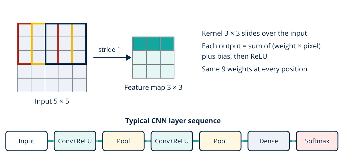
Convolutional neural networks (CNNs) are deep learning models built for grid data such as images. Small learned filters called kernels slide across the input to detect local patterns like edges and textures. Stacked convolution, activation and pooling layers build these into complex features, and final dense layers produce a classification or other output.
Convolutional neural networks power image classification, face recognition, medical image analysis, defect detection on production lines and the vision systems of self driving cars. They are a special kind of neural network whose structure matches the way images are organised: nearby pixels are related, and the same pattern can appear anywhere in the picture.
Why convolutional neural networks were needed
A 224 × 224 colour image has 224 × 224 × 3 = 150 528 input values. A fully connected layer with just 64 neurons would need over 9.6 million weights, and it would have to learn the same edge detector separately for every location. Goodfellow, Bengio and Courville describe three ideas that make convolution better suited:
- Sparse interactions: each output depends only on a small patch of the input, not on every pixel.
- Parameter sharing: the same kernel weights are used at every position, so a feature is learned once.
- Equivariance to translation: if the object moves in the image, its feature moves the same way in the feature map.
How a convolutional layer works
A kernel is a small grid of weights, typically 3 × 3 or 5 × 5, extending through all input channels. It is placed on a patch of the input, each weight is multiplied by the value under it, the products are summed and a bias is added. The kernel then slides by a step called the stride and repeats. The grid of results is a feature map. Strictly, deep learning libraries compute cross correlation (the kernel is not flipped), but it is still called convolution.
Stride, padding and output size
Padding adds a border of zeros around the input so that the kernel can be centred on edge pixels. With a 3 × 3 kernel, a padding of 1 and a stride of 1 keep the output the same size as the input (“same” padding). Without padding (“valid”) the output shrinks. For input width W, kernel size K, padding P and stride S, the output width is:
Channels and parameters
Each kernel spans all C_in input channels, so it has K × K × C_in weights plus one bias. A layer with C_out kernels produces C_out feature maps and has:
The number of parameters does not depend on the image size, which is the key saving compared with a dense layer.
Activation, pooling and dense layers
- Activation: after each convolution a nonlinear function, usually ReLU (max(0, x)), is applied element by element. Without it, stacked layers would collapse into one linear operation.
- Pooling: a max pooling layer takes the largest value in each small window, typically 2 × 2 with stride 2, halving the width and height. It reduces computation and makes features less sensitive to small shifts. Many modern networks use strided convolutions instead.
- Dense layers and output: at the end, feature maps are flattened or averaged (global average pooling) and passed to fully connected layers. A softmax output gives class probabilities.
Early layers learn simple features such as edges and colour blobs; deeper layers combine them into textures, parts and whole objects. Training uses backpropagation and gradient descent, like other neural networks, and needs care to avoid overfitting, usually with data augmentation, dropout and weight decay.
- Given
- A 224 × 224 × 3 colour image enters a convolutional layer with 64 kernels of size 3 × 3, stride 1 and padding 1, followed by 2 × 2 max pooling with stride 2.
- Find
- The output size of the convolution, its number of parameters, the size after pooling, and the weights a dense layer of 64 neurons would need on the same input.
- Assumptions
- One bias per kernel; no bias counted for the dense comparison.
- Solution
- W_out = (224 − 3 + 2 × 1) ÷ 1 + 1 = 224, so output is 224 × 224 × 64
N_params = (3 × 3 × 3 + 1) × 64 = 28 × 64 = 1792
After pooling: (224 − 2) ÷ 2 + 1 = 112, so 112 × 112 × 64
Dense layer: 150 528 × 64 = 9 633 792 weights - Answer
- Output 224 × 224 × 64 with only 1792 parameters, reduced to 112 × 112 × 64 by pooling; a dense layer would need about 9.6 million weights
- Limitations
- Parameters are few, but computation is not: the convolution still performs 224 × 224 × 64 × 27, about 86.7 million, multiply and add operations.
Key formulas for convolutional neural networks
| Quantity | Formula | Symbols and units |
|---|---|---|
| Output width (or height) | W_out = ⌊(W − K + 2P) ÷ S⌋ + 1 | W input size, K kernel size, P padding, S stride (pixels) |
| Parameters per conv layer | (K × K × C_in + 1) × C_out | C_in input channels, C_out number of kernels |
| Multiply and add operations | W_out × H_out × C_out × K × K × C_in | Per image, per layer |
| ReLU activation | f(x) = max(0, x) | Applied element by element |
| Pooling output (2 × 2, stride 2) | W_out = ⌊(W − 2) ÷ 2⌋ + 1 | Halves width and height |
Landmark CNN architectures
- LeNet-5 (1998): LeCun and colleagues used convolution and subsampling layers to read handwritten digits, establishing the basic CNN pattern.
- AlexNet (2012): trained on GPUs with ReLU and dropout, it won the ImageNet challenge with a top 5 error of 15.3%, against 26.2% for the next entry, and started the deep learning boom in vision.
- VGG (2014): showed that deep stacks of simple 3 × 3 convolutions work well.
- ResNet (2015): added skip (residual) connections that let the signal bypass layers, making networks of 152 layers trainable; it won the 2015 ImageNet challenge.
Applications of convolutional neural networks
CNNs are used for image classification, object detection and segmentation (compared in classification vs detection vs segmentation), optical inspection in machine vision systems, medical imaging, satellite image analysis and, in one dimensional form, vibration and sensor signals for predictive maintenance. In many vision tasks, transformer based models now compete with CNNs, and hybrid designs use both.
Convolutional neural networks interview and viva questions
- What is parameter sharing in a CNN? The same kernel weights are applied at every position of the input, so a feature is learned once and detected anywhere, with far fewer parameters.
- How do you calculate the output size of a convolutional layer? Use W_out = ⌊(W − K + 2P) ÷ S⌋ + 1, where W is input size, K kernel size, P padding and S stride.
- What does max pooling do? It keeps the largest value in each small window, reducing the spatial size and making features less sensitive to small shifts.
- Why is ReLU used after convolution? It adds nonlinearity so that stacked layers can learn complex functions, and it is cheap to compute.
- What problem do residual connections in ResNet solve? They let the signal and gradients bypass layers, which makes very deep networks easier to train.
Frequently asked questions
Why are CNNs better than ordinary neural networks for images?
A fully connected layer links every pixel to every neuron, which needs a huge number of weights and ignores the fact that nearby pixels are related. A convolutional layer uses small kernels that look at local patches and reuses the same weights at every position. This needs far fewer parameters and detects a feature wherever it appears in the image.
What is the difference between a kernel and a feature map?
A kernel (or filter) is the small grid of learned weights, such as 3 by 3, that slides over the input. A feature map is the output produced by sliding one kernel over the whole input, showing where in the image that kernel's pattern was found. A layer with 64 kernels produces 64 feature maps.
Are CNNs used only for images?
No. One dimensional CNNs are used for audio, sensor signals and time series such as vibration data, and CNNs are also used on spectrograms, text and other grid like data. Images are simply the best known application.
References
- I. Goodfellow, Y. Bengio and A. Courville, Deep Learning, MIT Press, 2016, Chapter 9 Convolutional Networks
- Y. LeCun, L. Bottou, Y. Bengio and P. Haffner, Gradient-based learning applied to document recognition, Proceedings of the IEEE, vol. 86, no. 11, 1998
- A. Krizhevsky, I. Sutskever and G. E. Hinton, ImageNet classification with deep convolutional neural networks, Advances in Neural Information Processing Systems 25, 2012
- K. He, X. Zhang, S. Ren and J. Sun, Deep residual learning for image recognition, IEEE Conference on Computer Vision and Pattern Recognition (CVPR), 2016
- V. Dumoulin and F. Visin, A guide to convolution arithmetic for deep learning, arXiv:1603.07285, 2016
Get one engineering email a week
New articles, worked examples and study notes every week. Free, no spam, unsubscribe any time.